Sunday, June 6, 2010
Final Lab: Mapping Census in ArcGIS
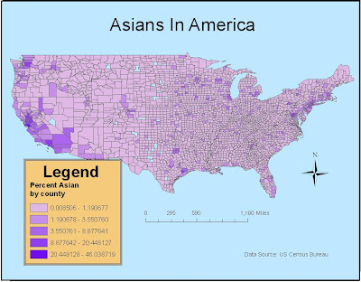
In the map examining the spatial distribution of Asian Americans in the United States, we see that the largest concentrations are in the Cities and areas surrounding San Francisco, Seattle, and New York. In general, the map shows that there are more Asians along the west coast than anywhere else in the country. This makes sense when you consider the geographical origins of Asian immigrants. In the late nineteenth and early twentieth century when a majority of immigration from Asia was going on they came over in large boats from the east looking for opportunity in America. It is also interesting that you see, in general, a larger proportion of Asians in urban areas. For example there are a bunch of cities where there is Asians surrounding it, but there are large concentrations in it like Chicago, Houston, and Dallas.
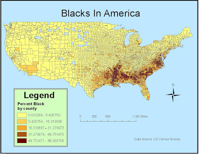
The map depicting the spatial distribution of Blacks in United States is much different from the map of Asian one. The concentrations of blacks in the far south, especially along the Mississippi River can be attributed to the history of slavery. The South was very invested in the slave trade from Africa which brought millions of black slaves over to work on the labor intensive plantations and farms in the south. We didn’t see this kind of involvement in the slave trade with the north because of a combination of moral and economic conflicts. Northern states were much more industrialized and urbanized than the south and the need for large scale labor operations was unnecessary. Even though the horrible history of slavery eventually did end, this didn’t affect where they were located and the large majority of blacks remained in the south after they were freed.
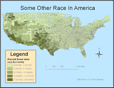
The map concerning the concentrations of other races in America is different from both of the other two maps. This category aggregates all people whose responses did not fall into the categories of “”White”, “Black or African American”, “American Indian and Alaska Native”, “Asian” and “Native Hawaiian and Other Pacific Islander”. This includes people who are half of a certain ethnicity like Asian, Mexican, Latino, Puerto Rican, Cuban, or something else more exotic. However, about 97% of this group is of Mexican descent. This explains the spatial distribution on the map. The highest proportions are in the southwest and California which corresponds with where most Mexican immigrants go. This makes sense when you consider the fact that most of them are either walking or driving from Mexico which borders the Southwestern portion of the United States on the southern border. There are also darker shades in the Southern portion of Florida. This is most likely a reflection of the large Cuban populations in the area.
From these maps, we can see that history and geography play a large role in the spatial distribution of ethnicities in the United States. They certainly are not dispersed evenly throughout the country and there are complex and unique reasons for their specific distributions. These maps are good for getting a general idea for where ethnicities are concentrated right now, but there they could be better if they were compared with other thematic maps that gave a map of how their distributions have changed over time or perhaps a comparison of spatial distributions of races and educational attainment or poverty. Essentially, these maps don’t actually work towards a point—they are more informative than anything.
GIS offers a way of visualizing data that would otherwise just be abstract numbers. Maps provide an instant picture that help us understand the spatial components of information. GIS also helps us bring disparate data sets together. For instance, a political campaign team could combine the thematic maps displaying ethnicity in America, as shown above, with maps of the electoral college to see where they should target their efforts. As an example, President Obama likely spent more time in the South than other presidents, knowing that he would have a good chance of getting out the black vote. Bill Richardson, the Governor of New Mexico who himself is half-Mexican, probably would have hit the campaign trail heavily in the Southwest were he to have conducted a national campaign. GIS helps us to easily see the relationships between people and places. GIS has other applications, too, whether in economics or environmental science, in politics or in the arts. With the click of a few buttons, we can develop a better understanding of the connections between the elements – like fire and rainfall, or between business factors like foot traffic and advertising. Just one computer program allows us the power to visualize knowledge in the form of maps, yet we must be aware of its flaws and of the limits of maps in general. People often view maps as “the truth” without questioning their validity. GIS can offer information in an attractive format, but its reliability depends upon the accuracy of the data source, the skills of the GIS technician, and the abilities of the cartographer to bring the various elements of a map together.
Thursday, May 27, 2010
Lab 7: Mapping the Station Fire in ArcGIS
On August 26, 2009, a massive fire broke out in Angeles National Forest, located in the northeastern portion of Los Angeles. The fire was christened the “Station Fire” due to its proximity to Mount Wilson, on top of which sits a station with 20 radio and television transmission towers. Firefighters were not able to completely contain the blaze until October 16, nearly two months later. The fire burned a total of 160,577 acres, making it the 10th largest in California state history. Unlike many other fires in Southern California, which are mostly grassland fires, the Station Fire was a true forest fire, as it burned primarily in the wooded hills of the Angeles National Forest. Still, the flames threatened homes in neighborhoods like La Canada Flintridge and Glendale, which border the forest to the south. 10,000 homes were evacuated as a precaution. In total, 64 structures were destroyed by the fire, and two firefighters were killed.
The first map is more a reference map than anything. I indicated the extents of the station fire on September 1st, the day with the largest area of fire coverage. It is layered on top of a map of Los Angeles with the census blocks designated. To spice it up a little bit, I also put the shaded block on a color scale indicating each blocs population density per square mile. The more red the bloc, the more people live in it. This allows someone looking at the map to immediately assess the where the areas of high concern are, purely in terms of the amount of people. Hopefully, the map allows viewers to see the extents of the fire in reference to the greater Los Angeles region. Sometimes, when you hear about something on the news it doesn’t actually hit home until you see how close you really were to the event. Someone living in the San Fernando Valley, for example, could see where their home is and then measure how close they were to the fire extents using the scale at the bottom and the map.
The Second map is a thematic map in that it looks at the same fire extents in the context of its proximity to children. The census blocs are shaded on a graded scale indicative of their population of children ages 5-17. To make the map easier to read, I put on a five mile buffer around the extents and then made it transparent so you could still see the census blocs. With this buffer you can see where the high concentrations of children that would be in danger are and respond accordingly for evacuations. As you can see on the map, the five mile radius includes the eastern portion of San Fernando, but more notably a fairly large residential population in Altadena. Using this map you can see where the largest risk areas for children are.
It’s important to examine where the largest populations of children are in relation to the fire, because all children are our future clichés aside, they are at a greater risk for smoke inhalation health issues. A New Jersey study showed that children represented a disproportionate percentage of people injured by smoke and fire. Children 11 and under comprised about ten percent of the population, but 22% of all fire related fatalities. With this in mind, it makes sense that neighborhoods with a high proportion of children plan for what to do in case of a fire—especially for those neighborhoods that are in close proximity to past fires. This would imply that the northern neighborhoods in Altadena and the eastern neighborhoods in San Fernando prepare accordingly for future fires as they lay within the buffer of the station fire.
In hindsight, high gusts and hot temperatures from the Santa Ana winds, contributed to the quick-burning blaze. The cause for the blaze, however, is thought to have been arson. The fire grew in size to an uncontrollable level in part because of the amount of dead, oily vegetable material on the ground, left over from decades of fire-free conditions. Such matter was highly combustible and provided fuel to the fire as it engulfed trees and wildlife alike. Thus, containing small fires will only lead to more massive, dangerous fires in the end. The Station Fire underscores the need for a reevaluation of California’s fire policy. Otherwise, only more fires will break out, and possibly even jump the line into the densely census tracts that you can see in the first map or worse yet to the neighborhoods with large child populations mentioned before.
California Department of Fire Protection.
http://cdfdata.fire.ca.gov/incidents/incidents_details_info?incident_id=377 (27 May 2010).
County of Los Angeles. "Station Fire Information."
http://www.lasdblog.org/Pressrelease/PR_Folder/SFUpdateTH-00.pdf.
InciWeb: Incident Information System.
http://www.inciweb.org/incident/1856/ (27 May 2010).
Lafferty, Kieth. "Smoke Inhilation." Web MD.
http://emedicine.medscape.com/article/771194-overview (27 May 2010).
Marciano, Rob. "'Angry fire' roars across 100,000 California acres." CNN.
http://www.cnn.com/2009/US/08/31/california.wildfires/index.html.
Thursday, May 20, 2010
Lab 6: DEM's in ArcGIS
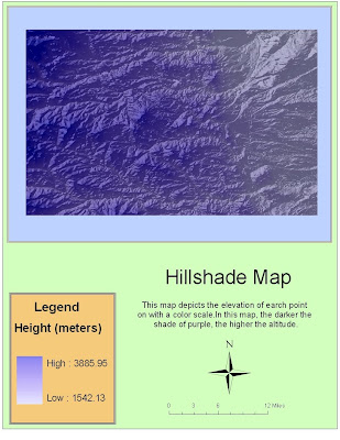
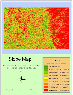
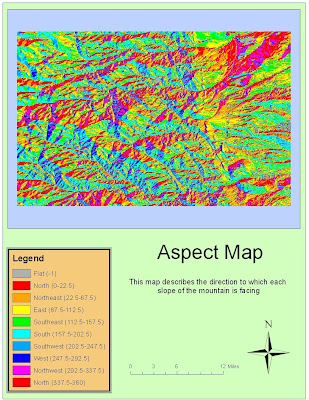
I chose a region in the Rockies of Colorado. This particular area is just to the West of Denver. There is a relative flatland on the eastern side of my region where the outskirts of the city are located. However, there is a pretty distinct north/south line where the higher elevations of the mountains become more evident. This is actually a region that I have been to and skied at so it was interesting seeing the area from this perspective. The geographic coordinate system used is the North American Datum S 1983.
The extents of the area of interest are:
Top 40.0427777773 degrees
Left -105.62861111 degrees
Right -105.113333332 degrees
Bottom 39.7141666661 degrees
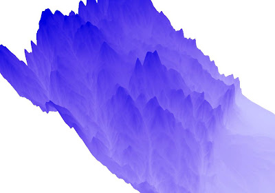
This last map is the 3D rendering of my area of interest. Hypothetically, it should give a three dimensional representation of the region I have been looking at for the last three maps.
Friday, May 14, 2010
Lab 5: Projections
The idea of map projections is a method for putting the sphere into two dimensional space. No matter how you do it these maps will be distorted. Generally, there are only really three ways to do try to do this. Your maps are either conformal, equidistant, or equal area. Conformal maps include projections like the Mercator or the North Pole Stereographic. They are intended to preserve angular relationships which is great in some situations (like navigation) and not as good in others. Equidistant projections like the Sinusoidal and the Plate Carree featured above intend to preserve distances between the origin and everything else on the map. Finally, equal area projections are meant to preserve the sizes of geographic features.
Conformal maps like the Mercator are probably the most common kind of map that you see in everyday life. It is used in classrooms, for reference, and for exploration. Its great because its relatively easy to make and read. However, it does distort the area closer to the poles. That’s why you see places like Greenland seeming so much larger than they really are. As a kid I thought Alaska was bigger than Mexico as a result of this distortion. Equidistant maps have a lot of positive features as well. For example, it’s the kind of map that you would want to use if you were measuring distance between points like Washington D.C. and Kabul for example. However, this only holds true if the points are of similar latitude in the Sinusoidal. If the straight line between the points is more diagonal then this kind of projection is more of a problem and you might want to use something like the Plate Carree which preserves distance along all latitudes. Equal Area maps like the Goode’s Homolosine projection is the best for maintaining the correct area of land masses. This way Greenland isn’t any bigger than it should be. However, it isn’t as good for comparing land features because it’s hard to represent the whole world as a rectangle.
Knowing the benefits and pitfalls of each of the types of projections, it becomes clear that there is no clear correct choice for maps. It is best to just choose your projection based on the circumstances and what your trying to convey. Nothing is going to preserve the correct comparative distance, shape, or area. Below are examples of each type of projection:
Conformal Maps
1: Mercator Projection: 10,112 miles
2: North Pole Stereographic Projection: 7,617 miles
Equidistant Mapping Projections
3: Sinusoidal: 8,098 miles
4: Plate Carree: 10,109 miles
Equal Area Maps
5: Lambert Azimuthal Equal Area: 6,806 miles
6: Goode’s Homolosine (Land): 9,986 miles
Thursday, May 6, 2010
Lab 4: Introducing ArcMap
I actually really enjoyed finally getting to use the ArcGIS software. We are going to start getting into the programs that we will be using for the majority of the GIS minor. I’m excited to get started and for that reason, going through that tutorial wasn’t as bad as I thought it was going to be. It seems like the possibilities are pretty incredible with ArcGIS as you are just able to do so much. That being said it really is another language so I was thankful for the well illustrated and easy to follow directions on the tutorial. The pictures highlighting exactly what to do made it easy for me to do the steps without getting stuck. It’s not exactly a aesthetically pleasing interface, but I suppose this isn’t really what’s important to ESRI. Function over form as the saying goes.
In the tutorial I created a printable page with four data frames on it: three maps and one chart. They were all related to a possible airport expansion. With the program, I was able to manipulate given data and shape files into a visually pleasant presentation of specific aspects related to the project. I thought it was particularly cool when I did the population density map and I was able, through the symbology tab, assign different colors to different levels of population density and spatially represent the data formerly only in table form. The program clearly has superior computing and graphing capabilities that other mapping software like say google maps just doesn’t have. I also think the tutorial made an effort to show all the wide array of different things you can do with ArcMap. While I don’t really know about other GIS software it seems like ArcMap is extremely versatile.
However being so versatile has its setbacks as well. The more capabilities a program has, the more confusing it’s going to be to learn. This unavoidable truth makes ArcMap’s depth both a blessing and a curse. I can tell this isn’t the kind of program that you can be an expert at after a few little tutorials. It takes hard work and lots and lots of practice to master software like this. To most working to learn the program will seem difficult and almost tedious. This is ok with me though because the less fun the program the more valued having the skill set will be.
I guess another setback for ArcGIS is that it has little potential for large scale public use. The combination of not being web 2.0 associated and the fact that it’s incredibly expensive makes it difficult for anyone outside a university or a company to recreationally use it. The bottom line is that this is essentially professional software that will always be complicated and difficult to use if you don’t know how. It will never be able to compete with up and coming web 2.0 phenomenon like google maps because to the average person it seems boring and difficult. This being said it’s an amazing group of software that I look forward to gaining expertise in and using it towards my career path.
Sunday, April 18, 2010
Lab 3: Neogeography
View Best Day Ever in a larger map
This is a map of what I like to imagine as the best day ever. I tried to make it relatively realistic in terms of how much I can accomplish and the feasibility of budget constraints, but it wouldn’t be the best day ever without a little extravagance right?
It doesn’t take too much brainpower to comprehend the usefulness of neogeography. It testifies to a time in history in which people are used to doing everything themselves. From personal computing, to social networking, to blogs we are indeed the do-it-yourself generation. Neogeography fits right into this mentality as it allows anyone, virtually anyone, to create maps for themselves or for others. It allows for unprecedented flexibility and individuality that map making used to lack. Being able to put additional information like pictures and videos into the map is helpful because you can enhance the message or desired ambiance of the map in ways that simple changes in colors and shapes can’t do. Being able to embed other websites into certain locations puts information at the tip of the viewers fingers if he/she so chooses to look.
However, there are a few pitfalls to neogeography as well. Purely based on my experience with Google My Maps there could be improvements in the existing software. I didn’t like how big each of the icons and their respective descriptions were. I feel like if there were any significant amount of icons the map would become cluttered and confusing. This is of course a rather petty complaint as far as pitfalls go. It is also possible that information shared on networks employing neogeography could be used in unintended ways. Although it is no complaint of the field or practice itself, it’s just important to be careful about what you make public because everyone can see and use the information for whatever intents and purposes they like. This includes criminals, sexual predators, stalkers and the like. This being said, as long as you are careful neogeography is incredibly helpful and has a bright future.
Wednesday, April 14, 2010
Lab 2
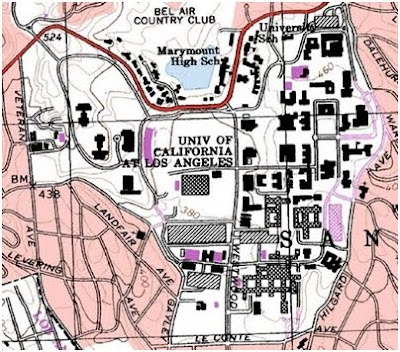
1. The quadrangle is called Beverly Hills
2. The adjasenct quadrangles are Hollywood, Burbank, Topanga, Van Nuys, Canoga Park, Venice, are Inglewood.
3. The quadrangle first created in 1966.
4. The North American Datum of 1927 was used to create this map.
5. The Scale is 1 : 24000
6. At the above scale, answer the following:
a) 5 centimeters on the map is equivalent to how many meters on the ground? A: 1200 meters.
b) 5 inches on the map is equivalent to how many miles on the ground? A: 1.89 miles
c) one mile on the ground is equivalent to how many inches on the map? A:. 2.64 inches
d) three kilometers on the ground is equivalent to how many centimeters on the map? 12.5 cm
7. What is the contour interval on your map? A: 20ft
8. What are the approximate geographic coordinates in both degrees/minutes/seconds and decimal degrees of:
a) the Public Affairs Building;
34.07403°, -118.43916°
34° 4′ 26.508″N, -118° 26′ 20.976″W
b) the tip of Santa Monica pier;
34.00748°, -118.49994°
34° 0′ 26.928″N, 118° 29′ 59.7834″W
c) the Upper Franklin Canyon Reservoir;
34.12046°, -118.41012°
34° 7′ 13.656″N, -118° 24′ 36.432″
9. What is the approximate elevation in both feet and meters of:
a) Greystone Mansion (in Greystone Park); 560 ft 170 meters
b) Woodlawn Cemetery; 140ft or 42.7 meters
c) Crestwood Hills Park; 620ft or 118 meters
10. What is the UTM zone of the map? 11.
11. What are the UTM coordinates for the lower left corner of your map?
UTM easting 3763000
UTM northing 362000
12. How many square meters are contained within each cell (square) of the UTM gridlines? 1,000,000 square meters.
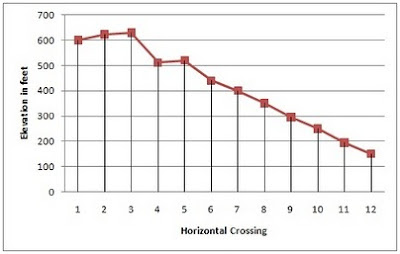
13. Obtain elevation measurements, from west to east along the UTM northing 3771000, where the eastings of the UTM grid intersect the northing. Create an elevation profile using these measurements in Excel (hint: create a line chart). Figure out how to label the elevation values to the two measurements on campus. Insert your elevation profile as a graphic in your blog.
14. The map has a 1999 magnetic declination north at the center of the map.
15. In which direction does water flow in the intermittent stream between the 405 freeway and Stone Canyon Reservoir? A: It flows North to South.
16.
Thursday, April 1, 2010
Lab 1: Three Maps
This is a population density map of the United States that I obtained from the Census information in 2000. Whoever made this map assigned a shade of red to correspond with the population density of the county. The darker the shade of red, the more people that live in that particular county. I think maps like this are interesting for a couple reasons. Most importantly, it's definitely important to know where the people of this country primarily live. As is pretty obvious from the map, centers of population are highly skewed to the east with only pockets of densely populated regions in the west such as the Denver area, the Pacific Northwest, the San Francisco Bay area, and Southern California. This is important to keep in mind as centers of population often determine political, social, and cultural importance. In the context of this map you can see why so many national organizations, sports teams, and economic activities are located in the east.
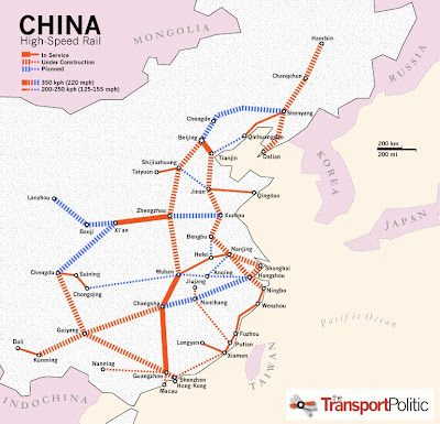
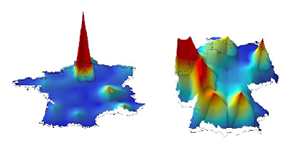
This is a map of the Chinese high speed rail network that I found in an article of the Transport Politic, which, as you might have guessed, is a transit oriented publication. The article, written by Yonah Freemark, tries to highlight the incredible public infrastructure investment China has been and is undergoing in the recent decade--particularly in high speed rail. As the map shows, the network isn't particularly impressive compared to other high speed rail power houses like France, Germany, or Spain in respects to their completed rail lines. However, when you consider all of the planned lines and the lines that are already under construction, China suddenly becomes a web of interconnected rail lines. You will soon be able to travel from Beijing in the north to Shanghai and even Hong Kong in the south all on efficient and cheap high speed rail lines. The map also shows the relative maximum speed of these lines by the width of the line on the map. In my opinion, this is an informative, well constructed map.This final map is taken from a weblog called the Map Room where they map the world’s economic activity on a one-degree grid. Animations for the entire globe are available, as are maps of individual countries. This particular map juxtaposes France's (on the left) spatial distribution of economic activity against Germany's (on the right). In areas of higher economic activity, the map appears to elevate and become more red. This is not a measure of population, although, as you can see, there is a fairly significant correlation between the two if you are familiar with where most of the two countries' populations are located. I think this map is really interesting because it highlights France's incredible economic reliance on Paris in relation to other parts of the country. This is in contrast to Germany's map which is relatively spread out in comparison. While the quality of these maps isn't particularly impressive, the information that they convey is definitely really interesting and it makes me want to know more about the reasons for such a difference in the two countries' spatial distribution of economic activity.
Subscribe to:
Posts (Atom)